Import Locations
8 minute read
OpenDataBio is distributed with a seed location dataset for Brazil, which includes state, municipality, federal conservation units, indigenous lands and the major biomes.
Working with spatial data is a very delicate area, so we have attempted to make the workflow for inserting locations as easy as possible.
If you want to upload administrative boundaries for a country, you may also just download a geojson file from OSM-Boundaries and upload it through the web interface directly. Or use the GADM repository exemplified below.
Importation is straightforward, but the main issues to keep in mind:
- OpenDataBio stores the geometries of locations using Well-known text (WKT) representation.
- Locations are hierarchical, so a location SHOULD lie completely within its parent location. The importation method will try to detect the parent locations based on its geometry. So you do not need to inform a parent. However, sometimes the parent and child locations share a border or have minor differences that prevent to be detected. Therefore, if this importation fail to place the location where you expected, you may update or import informing the correct parent. When you inform the parent a second check will be performed adding a buffer to the parent location, and should solve the issue.
- Country borders can be imported without parent detection or definition, and marine records may be linked to a parent even if they are not contained by the parent polygon. This requires a specific field specification and should be used only in such cases as it is a possible source of misplacement, but give such flexibility)
- Standardize the geometry to a common projection of use in the system. Strongly recommended to use EPSG:4326 WGS84., for standardization;
- Consider, uploading your political administrative polygons before adding specific POINT, PLOTS or TRANSECTS;
- Conservation Units, Indigenous Territories and Environmental layers may be added as locations and will be treated as special case as some of these locations span different administrative locations. So a POINT, PLOT or TRANSECT location may belong to a UC, a TI and many Environmental layers if these are stored in the database. These related locations, like the political parent, are auto-detected from the location geometry.
Check the POST Locations API docs in order to understand which columns can be declared when importing locations.
Adm_level defines the location type
The administrative level (adm_level) of a location is a number:
- 2 for country; 3 to 10 as other as ‘administrative areas’, following OpenStreeMap convention to facilitate external data importation and local translations (TO BE IMPLEMENTED). So, for Brazil, codes are (States=4, Municipalities=8);
- 999 for ‘POINT’ locations like GPS waypoints;
- 101 for transects
- 100 is the code for plots and subplots;
- 99 is the code for Conservation Units
- 98 for Indigenous Territories
- 97 for Environmental polygons (e.g. Floresta Ombrofila Densa, or Bioma Amazônia)
Importing spatial polygons
GADM Administrative boundaries
Administrative boundaries may also be imported without leaving R, getting data from GDAM and using the odb_import* functions
library(raster)
library(opendatabio)

#download GADM administrative areas for a country

#get country codes
crtcodes = getData('ISO3')
bra = crtcodes[crtcodes$NAME%in%"Brazil",]

#define a path where to save the downloaded spatial data
path = "GADMS"
dir.create(path,showWarnings = F)

#the number of admin_levels in each country varies
#get all levels that exists into your computer
runit =T
level = 0
while(runit) {
   ocrt <- try(getData('GADM', country=bra, level=level,path=path),silent=T)
   if (class(ocrt)=="try-error") {
      runit = FALSE
   }
   level = level+1
}

#read downloaded data and format to odb
files = list.files(path, full.name=T)
locations.to.odb = NULL
for(f in 1:length(files)) {
   ocrt <- readRDS(files[f])
   #class(ocrt)
   #convert the SpatialPolygonsDataFrame to OpenDataBio format
   ocrt.odb = opendatabio:::sp_to_df(ocrt)  #only for GADM data
   locations.to.odb = rbind(locations.to.odb,ocrt.odb)
}
#see without geometry
head(locations.to.odb[,-ncol(locations.to.odb)])

#you may add a note to location
locations.to.odb$notes = paste("Source gdam.org via raster::get_data()",Sys.Date())

#adjust the adm_level to fit the OpenStreeMap categories
ff = as.factor(locations.to.odb$adm_level)
(lv = levels(ff))
levels(ff) = c(2,4,8,9)
locations.to.odb$adm_level = as.vector(ff)

library(opendatabio)
base_url="https://opendb.inpa.gov.br/api"
token ="GZ1iXcmRvIFQ"
cfg = odb_config(base_url=base_url, token = token)
odb_import_locations(data=locations.to.odb,odb_cfg=cfg)

#ATTENTION: you may want to check for uniqueness of name+parent rather than just name, as name+parent are unique for locations. You may not save two locations with the same name within the same parent.
A ShapeFile example
library(rgdal)

#read your shape file
path = 'mymaps'
file = 'myshapefile.shp'
layer = gsub(".shp","",file,ignore.case=TRUE)
data = readOGR(dsn=path, layer= layer)

#you may reproject the geometry to standard of your system if needed
data = spTransform(data,CRS=CRS("+proj=longlat +datum=WGS84"))

#convert polygons to WKT geometry representation
library(rgeos)
geom = rgeos::writeWKT(data,byid=TRUE)

#prep import
names = data@data$name  #or the column name of the data
shape.to.odb = data.frame(name=names,geom=geom,stringsAsFactors = F)

#need to add the admin_level of these locations
shape.to.odb$admin_level = 2

#and may add parent and note if your want
library(opendatabio)
base_url="https://opendb.inpa.gov.br/api"
token ="GZ1iXcmRvIFQ"
cfg = odb_config(base_url=base_url, token = token)
odb_import_locations(data=shape.to.odb,odb_cfg=cfg)
Converting data from KML
#read file as SpatialPolygonDataFrame
file = "myfile.kml"
file.exists(file)
mykml = readOGR(file)
geom = rgeos::writeWKT(mykml,byid=TRUE)

#prep import
names = mykml@data$name  #or the column name of the data
to.odb = data.frame(name=names,geom=geom,stringsAsFactors = F)

#need to add the admin_level of these locations
to.odb$admin_level = 2

#and may add parent or any other valid field

#import
library(opendatabio)
base_url="https://opendb.inpa.gov.br/api"
token ="GZ1iXcmRvIFQ"
cfg = odb_config(base_url=base_url, token = token)
odb_import_locations(data=to.odb,odb_cfg=cfg)
Import Plots and Subplots
Plots and Transects are special cases within OpenDataBio:
- They may be defined with a Polygon or LineString geometry, respectively;
- Or they may be registered only as POINT locations. In this case OpenDataBio will create the polygon or linestring geometry for you;
- Dimensions (x and y) are stored in meters
- SubPlots are plot locations having a plot location as a parent, and must also have cartesian positions (startX, startY) within the parent location in addition to dimensions. Cartesian position refer to X and Y positions within parent plot and hence MUST be smaller than parent X and Y. And the same is true for Individuals within plots or subplots when they have their own X and Y cartesian coordinates.
- SubPlot is the only location that may be registered without a geographical coordinate or geometry, which will be calculated from the parent plot geometry using the startx and starty values.
Plot and subplot example 01
You need at least a single point geographical coordinate for a location of type PLOT. Geometry (or lat and long) cannot be empty.
#geometry of a plot in Manaus
southWestCorner = c(-59.987747, -3.095764)
northWestCorner = c(-59.987747, -3.094822)
northEastCorner = c(-59.986835,-3.094822)
southEastCorner = c(-59.986835,-3.095764)
geom = rbind(southWestCorner,northWestCorner,northEastCorner,southEastCorner)
library(sp)
geom = Polygon(geom)
geom = Polygons(list(geom), ID = 1)
geom = SpatialPolygons(list(geom))
library(rgeos)
geom = writeWKT(geom)
to.odb = data.frame(name='A 1ha example plot',x=100,y=100,notes='a fake plot',geom=geom, adm_level = 100,stringsAsFactors=F)
library(opendatabio)
base_url="https://opendb.inpa.gov.br/api"
token ="GZ1iXcmRvIFQ"
cfg = odb_config(base_url=base_url, token = token)
odb_import_locations(data=to.odb,odb_cfg=cfg)
Wait a few seconds, and then import subplots to this plot.
#import 20x20m subplots to the plot above without indicating a geometry.
#SubPlot is the only location type that does not require the specification of a geometry or coordinates,
#but it requires specification of startx and starty relative position coordinates within parent plot
#OpenDataBio will use subplot position values to calculate its geographical coordinates based on parent geometry
(parent = odb_get_locations(params = list(name='A 1ha example plot',fields='id,name',adm_level=100),odb_cfg = cfg))
sub1 = data.frame(name='sub plot 40x40',parent=parent$id,x=20,y=20,adm_level=100,startx=40,starty=40,stringsAsFactors=F)
sub2 = data.frame(name='sub plot 0x0',parent=parent$id,x=20,y=20,adm_level=100,startx=0,starty=0,stringsAsFactors=F)
sub3 = data.frame(name='sub plot 80x80',parent=parent$id,x=20,y=20,adm_level=100,startx=80,starty=80,stringsAsFactors=F)
dt = rbind(sub1,sub2,sub3)
#import
odb_import_locations(data=dt,odb_cfg=cfg)
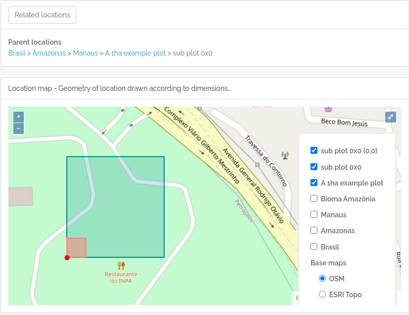
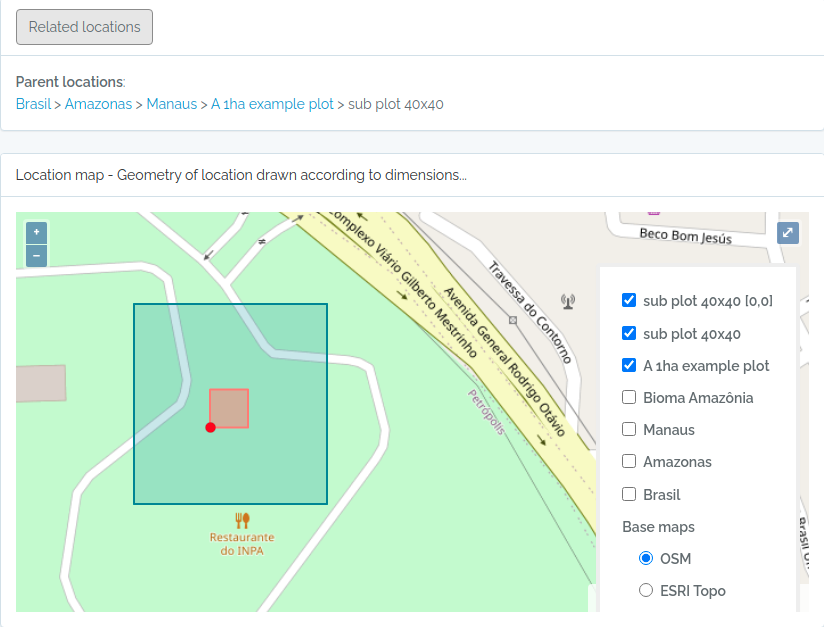
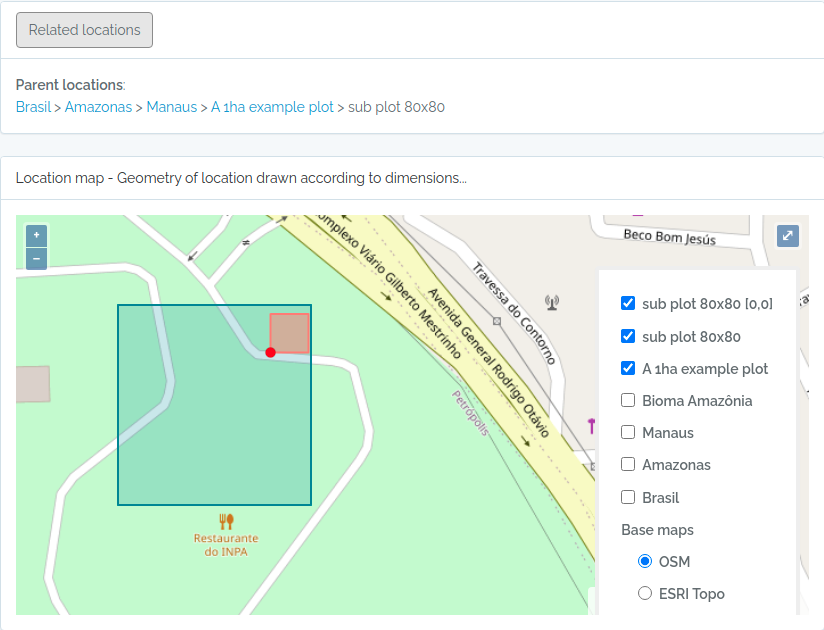
Screen captures of imported plots
Below screen captures for the locations imported with the code above
Plot and subplot example 02
Import a plot and subplots having only:
- a single point coordinate
- an azimuth or angle of the plot direction
library(opendatabio)
base_url="https://opendb.inpa.gov.br/api"
token ="GZ1iXcmRvIFQ"
cfg = odb_config(base_url=base_url, token = token)
#the plot
geom = "POINT(-59.973841 -2.929822)"
to.odb = data.frame(name='Example Point PLOT',x=100, y=100, azimuth=45,notes='OpenDataBio point plot example',geom=geom, adm_level = 100,stringsAsFactors=F)
odb_import_locations(data=to.odb,odb_cfg=cfg)
#define 20x20 subplots cartesian coordinates
x = seq(0,80,by=20)
xx = rep(x,length(x))
yy = rep(x,each=length(x))
names = paste(xx,yy,sep="x")
#import these subplots without having a geometry, but specifying the parent plot location
parent = odb_get_locations(params = list(name='Example Point PLOT',adm_level=100),odb_cfg = cfg)
to.odb = data.frame(name=names,startx=xx,starty=yy,x=20,y=20,notes="OpenDataBio 20x20 subplots example",adm_level=100,parent=parent$id)
odb_import_locations(data=to.odb,odb_cfg=cfg)
#get the imported plot locations and plot them using the root parameter
locais = odb_get_locations(params=list(root=parent$id),odb_cfg = cfg)
locais[,c('id','locationName','parentName')]
colnames(locais)
for(i in 1:nrow(locais)) {
geom = readWKT(locais$footprintWKT[i])
if (i==1) {
plot(geom,main=locais$locationName[i],cex.main=0.8,col='yellow')
axis(side=1,cex.axis=0.7)
axis(side=2,cex.axis=0.7,las=2)
} else {
plot(geom,add=T,border='red')
}
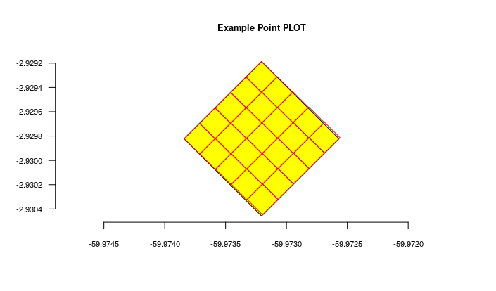
}
The figure generated above:
Import transects
This code will import two transects, when defined by a LINESTRING geometry, the other only by a point geometry. See figures below for the imported result
#geometry of transect in Manaus

#read trail from a kml file
  #library(rgdal)
  #file = "acariquara.kml"
  #file.exists(file)
  #mykml = readOGR(file)
  #library(rgeos)
  #geom = rgeos::writeWKT(mykml,byid=TRUE)

#above will output:
geom = "LINESTRING (-59.9616459699999993 -3.0803612500000002, -59.9617394400000023 -3.0805952900000002, -59.9618530300000003 -3.0807376099999999, -59.9621049400000032 -3.0808563200000001, -59.9621949100000009 -3.0809758500000002, -59.9621587999999974 -3.0812666800000001, -59.9621092399999966 -3.0815010400000000, -59.9620656999999966 -3.0816403499999998, -59.9620170600000009 -3.0818584699999998, -59.9620740699999999 -3.0819864099999998)";

#prep data frame
#the y value refer to a buffer in meters applied to the trail
#y is used to validate the insertion of related individuals
to.odb = data.frame(name='A trail-transect example',y=20, notes='OpenDataBio transect example',geom=geom, adm_level = 101,stringsAsFactors=F)

#import
library(opendatabio)
base_url="https://opendb.inpa.gov.br/api"
token ="GZ1iXcmRvIFQ"
cfg = odb_config(base_url=base_url, token = token)
odb_import_locations(data=to.odb,odb_cfg=cfg)

#NOW IMPORT A SECOND TRANSECT WITHOUT POINT GEOMETRY
#then you need to inform the x value, which is the transect length
#ODB will map this transect oriented by the azimuth paramater (south in the example below)
#point geometry = start point
geom = "POINT(-59.973841 -2.929822)"
to.odb = data.frame(name='A transect point geometry',x=300, y=20, azimuth=180,notes='OpenDataBio point transect example',geom=geom, adm_level = 101,stringsAsFactors=F)
odb_import_locations(data=to.odb,odb_cfg=cfg)

locais = odb_get_locations(params=list(adm_level=101),odb_cfg = cfg)
locais[,c('id','locationName','parentName','levelName')]
The code above will result in the following two locations:
![]()
![]()